Fast method to interpolate scattered data onto a rectangular grid for visualization purposes

Introduction

When studying a set of data samples with the intention to get insight into approximate shapes, it helps very much to display a continuous field of values instead of the individual scattered data points. Numerous interpolation methods have been developed, often starting from Delaunay triangulation for handling the spatial distribution between points. These methods generally deliver high accuracy at the expense of computation speed, storage requirements, and/or algorithmic complexity.

Different trade-offs are possible, especially when it is not vitally important to obtain high accuracy. Also, when it is known that a visualization will be rendered onto a rectangular grid, such as a color-coded bitmap picture or a 3D mesh plot, specific characteristics can be exploited.

The easily implemented algorithm described below, will provide useful interpolation results at O(p) complexity in both computation and storage, where p is the number of grid points (pixels) in the interpolation result. It is assumed that the number of data samples n will be lower than the number of display pixels p; otherwise interpolation would not be required anyway. Yet the method will continue to work equally efficiently even for very large numbers of data samples.

General concept

The basic flow for determining any interpolated value is as follows:

1. Find a set of nearby data samples ("close neighbors");

2. Compute the interpolated value, based on values of (and distances to) these neighbors.

In the method described below, "close neighbors" are chosen to be the nearest data samples in each of eight direction segments. This gives a maximum of eight neighbors that are guaranteed to be spread out spatially. No limit is imposed on distance, specifically to allow for smooth interpolation between a large number of nearby data samples in one direction and some far-away data samples in an opposite direction. The neighbor samples are then combined using inverse distance weighting to obtain the interpolated value.

Neighbor samples are never searched for, starting from each interpolated pixel. Rather, all data samples are expanded into each of the eight direction segments. This can be implemented very efficiently thanks to the rectangular grid structure, and is executed for the entire grid in one linear pass per direction segment, also calculating the inverse distance weights immediately. After that, all eight close neighbors plus weights will be present and waiting for all grid points, leaving only the summation to be done.

So the actual implementation is as follows:

1. Expand all data samples into the eight direction segments, including inverse distance calculation;

2. For each grid point, compute the weighted sum of the expanded data sample values at that grid point.

Note that this method will select just one data sample from any direction segment, even if many samples would be available there. The assumption is that the underlying data is "smooth" compared to the sample pattern, and that considering multiple clustered samples would not add much information. Actually, it would cause the inverse distance weighting to become skewed towards that particular direction, just because of the spatial distribution of the samples, which would be quite undesirable. Indeed, an intended use case for this method is for data samples that are not randomly distributed but highly clustered.

As a matter of convenience, all data sample locations are rounded to exact grid points. This is acceptable because maximum accuracy is not required, and the chosen grid spacing is assumed to provide the desired detail level. In case multiple data samples are rounded to the same grid point, they may be averaged, or used according to first or last arrival. This means that all grid points either have one data sample ready, or need interpolation where the closest neighbor is at least one grid spacing away.

Expanding data

The figure below shows a grid point P, to be interpolated from eight nearby data samples D. These data samples D are the nearest in each of the eight direction segments as seen from P. Also shown are some other data samples (d) that are further away in their respective segments, so they will not be considered.

The main observation is that some data sample D will be the nearest in the West-South-West direction as seen from some interpolation point P, if and only if P is located in the East-North-East "influence region" of D. That "influence region" ends whenever any other data sample's "influence region" takes over. When starting from P, it is relatively hard to search for D choices; but when starting from D, it is straightforward to extend "influence regions".

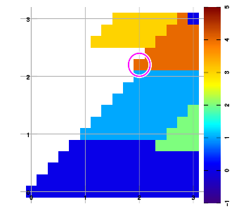
Above figure b) shows an example expansion for three data samples (red, blue, green), halfway through execution. To extend into the East-North-East direction, the grid is traversed starting from the bottom row, left to right, then the next higher row, left to right, and so on. Grid points are left "empty" (valueless) whenever no data sample has been encountered yet since starting that row.

When considering each grid point, the two possibilities are:

1. The grid point has a data sample itself; then use it. For the weight, choose any number. (The grid point will get the same data sample and the same weight in all expansion directions).

2. The grid point has no data sample. Then there are two candidate samples:

   a. the sample that was extended into the grid point immediately left;

   b. the sample that was extended into the grid point left-below.

   For both candidates, calculate the distance to the original data sample, then choose the one which is closest. This also immediately produces the inverse distance weight.

   (Either or both candidates may be empty, then the choice is trivial.)

   Given that this expansion considers one direction segment only, there can be no other data samples that may have any influence except these two.

The results for this East-North-East expansion are stored into a dedicated grid "layer" for later reference.

All other seven directions can be expanded in the same way, by varying the row-first vs. column-first and "forward" vs. "backward" directions. Results are stored in seven other grid layers.

The complete execution will always have a fixed number of eight passes along all grid points, doing a fixed calculation concerning (at most) two data sample locations for each grid point. The eight directions are fully independent, and may be calculated in parallel on multi-processing systems.

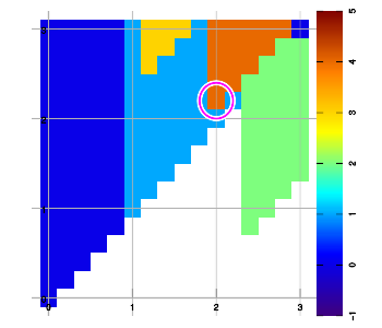
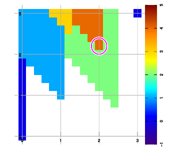
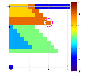
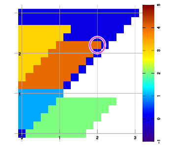
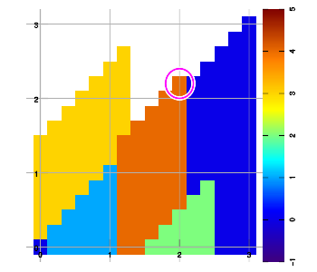
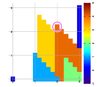
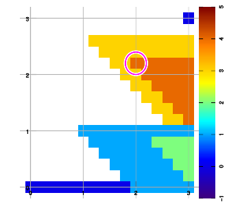
Below are example plots for expansion of a set of six data points in all eight directions. Two points are located at corners to set up the graphic area. As an artifact of the implementation, a magenta marker surrounds the most recently added data sample.

Combining layers

A final pass over all grid points is needed to combine the eight direction layers at each grid point. This is almost as simple as calculating the weighted sum using the data samples and weights that are waiting in the eight layers.

However, some special care is needed to skip "empty" values where no data sample was available in that direction. Further, as can be seen in the examples above, the expansion has the characteristic of always including both the straight edge and the diagonal edge. This may cause the same data sample to be selected for two adjacent direction segments whenever the interpolating point is in a straight or diagonal line from a data sample. De-duplication must be applied to prevent any data sample from being included twice.

This final pass is completely independent for all grid points, and may be parallellized as desired.

Boundaries

When expanding data samples into the eight separate direction segments, spatial limiting must be imposed to prevent gross extrapolations outside of the original data sample space. The smallest rectangle surrounding the sample points is very suitable to limit the grid itself, and is easily obtained from registering minimum and maximum sample coordinates.

A further spatial limiting is easily applied during the "combining" stage: if any interpolation point has no value in four (or more) consecutive segments, then it must certainly be outside of the data sample space. This will give an outer shape that somewhat resembles an octagon, which will be slightly larger than the convex hull.

In cases where only very few data samples are available, there is some "risk" of extrapolation inside the sample area, namely when too few direction segments provide any value. If desired, this can also be checked in the "combining" stage.

Dimensionality

The two-dimensional algorithm as discussed, applies trivially in one dimension by expanding data samples only to the left and to the right on the number line, until a next data sample is encountered.

The two-dimensional version itself can be simplified by considering only four "90-degrees" direction segments (NW, SW, SE, NE). In the given expansion algorithm, this is easily implemented by considering candidate grid points immediately left and immediately below. For two dimensions, this is not advised since the resulting interpolation set will be unnecessarily limited.

Yet for three dimensions, this simplified "90-degrees" expansion is very useful, and it will provide "boxed" expansions in eight directional segments.

The algorithm still applies in four or more dimensions. However, properly visualizing any rectangular grid will quickly become challenging. Using "90-degrees" expansion, one directional segment will result for any combination of the grid axes traversed in both directions, i.e. 2^d for d dimensions. This compares favorably to the number of grid points that is also expected to grow by d power in order to remain useful.

Examples

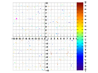
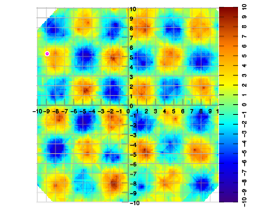
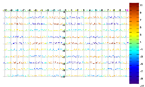
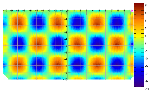
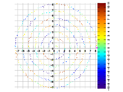
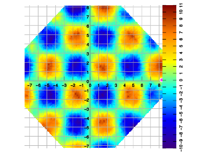
All examples below were created by sampling the same function f(x,y) = 10 * sin(x) * sin(y).

Example 1. Set of 400 data samples at random locations, vs. interpolated result. The sample density is quite lower than the intended application, and even lower than the Nyquist criterion in some areas. This gives an impression of the artifacts as generated by the interpolation method, which is specifically not designed to be maximally accurate.

The following examples more closely match expected real-world scenarios for the intended application.

Example 2. Data sampled in linear walks, vs. interpolated result.

Example 3. Data sampled in spiral walk, vs. interpolated result.

This document is Copyright © 2021 J.A.Bezemer@opensourcepartners.nl, licensed under GNU GPL >=3.

Any implementation of the algorithm will be governed by its own license.